Read in Data From a Url in R
You can probably retrieve of "reading matter" as beingness 1 of three sorts:
- data
- R objects
- scripts
Data is a general term and by this I hateful numbers and characters that you might reasonably suppose could be handled past a spreadsheet. Your information are what you use in your analyses.
R objects may exist data or other things, such as custom R commands. They are normally stored (on disk) in a format that tin can just be read by R simply sometimes they may be in text form.
Scripts are collections of R commands that are designed to be run "automatically". They are generally saved (on disk) in text format.
Reading – using the keyboard
The simplest way to "read" data into R is to type information technology yourself using the keyboard. The c() command is the simplest method. Recollect of c for "combine" or "concatenate". To make some data you lot type them in the control and split the elements with commas:
> dat1 <- c(ii, 3,4,5, 7, 9) > dat1 [i] 2 iii four v 7 nine
Notation that R ignores any spaces.
If you desire text values you will have to enclose each chemical element in quotes, y'all can utilise unmarried or double quotes as long as they "friction match".
> dat2 <- c("Kickoff", 'Second', "Third") > dat2 [1] "First" "2d" "3rd" When you "display" your text (graphic symbol) information R includes the quotes (R always shows double quotes). You can utilise the c() command to join many items, non only numbers or character data. However, here you'll see it used simply for "reading" regular data. The result of the c() control is generally a vector, a i-dimensional information object. You tin add together to existing data merely if yous "mix" information types you may not get what yous expect:
> dat3 <- c(ane, 2, iii, "Kickoff", "2d", "3rd") > dat3 [ane] "i" "2" "iii" "First" "2nd" "Third"
R has converted the numbers to text (character) values.
Use scan()
Typing the commas and/or quotes tin be a pain, especially when you have more than a few items to enter. This is where the browse() command comes in useful. The scan() command is quite flexible and can read the keyboard, clipboard and files on disk. The simplest manner to employ scan() is for entering numbers. Yous invoke the command and then type numerical values, separated by spaces. You lot can press the ENTER primal at whatsoever time just the data entry will non terminate until you press ENTER on a blank line (i.eastward. you lot press ENTER twice).
> dat4 <- scan() i: 3 6 7 12 13 ix viii 4 9: seven vii eight 12 5 14: four 15: Read 14 items
> dat4 [1] 3 6 7 12 13 9 eight 4 vii 7 8 12 five iv
In the preceding instance 8 values were typed then the ENTER pressed. Y'all can see that the R cursor changes from the >. This helps you to keep track of how many items yous've typed. Subsequently the start eight items we typed five more (the line beginning with 9:) and then pressed ENTER over again. R displayed xiv: to show us that the next item would be the 14th. One value was typed and then ENTER pressed twice to consummate the process.
If you lot desire to type grapheme data you lot must add the what = "grapheme" parameter to the command, and so R "knows" what to look and you exercise not demand to type quotes:
> dat5 <- browse(what = "character") 1: Mon Tue Wed Thu Fri 6: Sat Sun 8: Read 7 items
> dat5 [one] "Mon" "Tue" "Wed" "Thu" "Fri" "Sat" "Dominicus"
You lot tin specify the separator character using the sep = parameter, although the default space seems adequate! If you are then inclined, you can also specify an alternative character for the decimal point via the dec = parameter.
> dat6 <- scan(sep = "", dec = ",") 1: 34 4,six three: 1,4 7,34 5: Read 4 items > dat6 [1] 34.00 4.60 ane.40 7.34
Notice that the default is actually ii quotes with no space between! The sep and dec parameters are more than useful for reading data from clipboard or disk files, as you lot will come across next.
Reading – using the clipboard
The browse() control can read the clipboard. This tin be useful to shift larger quantities of data into R. Y'all'll probably have data in a spreadsheet but any programme that tin display text volition let yous to copy to the clipboard.
Information in a spreadsheet
If you open the data is a spreadsheet and so you can copy a column of information and apply scan() as if you lot were going to type it from the keyboard. Yous exercise not need to specify the separator character (the default "" will suffice) when using a spreadsheet but you lot tin specify the decimal point character if necessary.
Opening a text file in Excel allows you to encounter the data separator.
If you need to re-create items by row, then you cannot do it using a spreadsheet unless y'all accept a Mac. To get a column of information into R you simply copy the data to the clipboard:


If y'all demand to copy items by row, and then you cannot do it using a spreadsheet unless yous have a Mac. To get a column of data into R you merely copy the data to the clipboard:
So switch to R and use the scan() command:
> dat7 <- scan() 1: 34 2: 32 3: 30 4: 36 5: 36 6: 36 7: 41 8: 35 9: 30 10: 34 11: Read 10 items
To finish you lot printing ENTER on a blank line, this means yous could copy more data and append it if you wish.
Multiple paste
In one case you've pasted some information into R using scan() you finish the operation past pressing ENTER on a bare line. Unremarkably this ways that you lot have to press ENTER twice. If yous desire to add more data, you can just press ENTER in one case and re-create/paste more stuff.
Rows of information
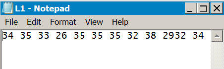
If the data are in a spreadsheet or are separated past TAB characters you cannot read rows of information (unless you lot have a Mac). If yous open the data in a text editor (Notepad or Wordpad for instance) then you'll be able to select and re-create multiple rows of data as long as the items are not TAB separated. In the following example Notepad is used to open a comma separated file. Several rows are copied to the clipboard:

The browse() command tin can now be used, using the sep = "," parameter equally the data are comma separated:
> dat8 <- scan(sep = ",")
i: 34,35,33,26,35,35,35,32,38,29
eleven: 32,34,33,29,37,37,31,37,31,28
21: xxx,38,34,33,33,32,29,35,29,30
31:
Read xxx items
In total 30 information elements were read (note that the data are read row by row). ENTER was pressed after the first paste operation simply you could add more data, completing data entry by pressing ENTER on a blank line.
End of Line characters
Text files can be split into lines using several methods. In general Linux and Mac use LF whereas Windows uses CR/LF (older Mac used CR). This can mean that if you apply Windows and Notepad to open a file the information are not displayed "neatly" and everything appears on 1 line.
Wordpad is built in to Windows and this will handle alternative line endings quite fairly.
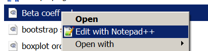
The Notepad++ program will also handle culling stop of line characters and allows y'all to alter the EOL setting for a file. It also supports syntax highlighting.

On a Mac the default TextEdit app volition deal with alternative line endings but BBEdit is a useful editor, which also supports syntax highlighting.
If you use Linux, then it is probable that your default text editor will bargain with any EOL setting and also let you to alter the encoding.
Converting separators

If y'all accept data in TAB separated format and want to convert information technology to elementary space separated or comma separated format, so the easiest way is to open the data in your spreadsheet. Then applyFile > Save Equally.. to save the file in a new format.
The preceding example shows Excel 2010 only other versions of Excel have similar options. OpenOffice and LibreOffice likewise allow saving of files in various formats.
The TAB separated format is useful for displaying items for people to read but not and then skillful for re-create/paste. Comma separated files are more often than not almost useful and tin be produced past many programs. Space separated files are somewhere in-between.
Of course there is no need to convert TAB separated files, they are but a problem if you are going to use copy/paste. R can handle TAB separators quite hands if the file is to be read directly from disk.
Reading – from disk files
If yous have a information file on deejay, you can read it into R without opening it first. There are ii main options:
- the scan() command
- the table() command
More often than not speaking you'd use scan() to read a data file and make a vector object in R. That is, you utilise it to get/make a single sample (a one-D object). Y'all use the read.tabular array() command to access a file with multiple columns, each one representing a separate sample or variable. The event is a data.frame object in R (a 2-D object with rows and columns).
The read.table() command has many options and there are several convenience functions, such as read.csv(), allowing you to read some popular formats with appropriate defaults.
Use browse() to read a disk file
To get scan() to read a file from disk you but specify the filename (in quotes) in the control. You tin ready the separator character and decimal point character as advisable using sep = and dec = parameters. If you lot are using Windows or Mac yous can use file.cull() instead of the filename:
> dat8 <- browse(file.choose()) Read 100 items
The file.choose() office opens a browser-like window and permits you to select the file you lot crave.
The file selected in the preceding example was chosen L1.txt and you can view this in your browser. It is simply separated with spaces. The result is a vector of 100 data items even though the original file seems equanimous of ten columns.

If you have a file separated with commas, similar L2.txt, then you just specify sep = "," similar so:
> dat9 <- scan(file.choose(), sep = ",") Read 100 items
The result is the same, a vector of 100 items. When the separator character is a TAB (e.g. L3.txt) you lot can apply the sep = "\t" parameter.
> dat10 <- scan(file.choose(), sep = "\t") Read 100 items
Sometimes your information may include comments, these are helpful to remind you what the information were but yous need to be able to deal with them.
Comments in data files
It is helpful to include comments in plainly data files. This helps yous (and others) to determine what the data stand for without having to await elsewhere. The scan() control can "read and ignore" rows that are "flagged" every bit comments.
You can set up rows that brainstorm with a special character to be ignored using the comment.char = parameter. Of course you could utilize any character as a comment marker merely in R the # is used and so that would seem sensible.
> dat11 <- scan(file.cull(), comment.char = "#") Read 100 items
Have a look at the L1c.txt file. This has three annotate lines at the kickoff. The file itself is space separated.
Working directory
If you lot practise not apply file.cull() or yous have Linux Bone and so you'll have to specify the filename exactly (in quotes). R uses a working directory, where it stores files and where it looks for items to read. Yous can see the current working directory using getwd():
> getwd() [one] "/Users/markgardener" > getwd() [1] "C:/Users/Mark/Documents"
You can set the working directory to a new folder past specifying the new filepath (in quotes) in the setwd() command:
> getwd() # Go the current wd [1] "/Users/markgardener" > setwd("Desktop") # Set to new value > getwd() # Check that wd is set as expected [ane] "/Users/markgardener/Desktop" > setwd("/Users/markgardener") # set back to original > getwd() [i] "/Users/markgardener" You lot can "reset" your working directory using the tilde:
> setwd("~") > getwd() [1] "/Users/markgardener" 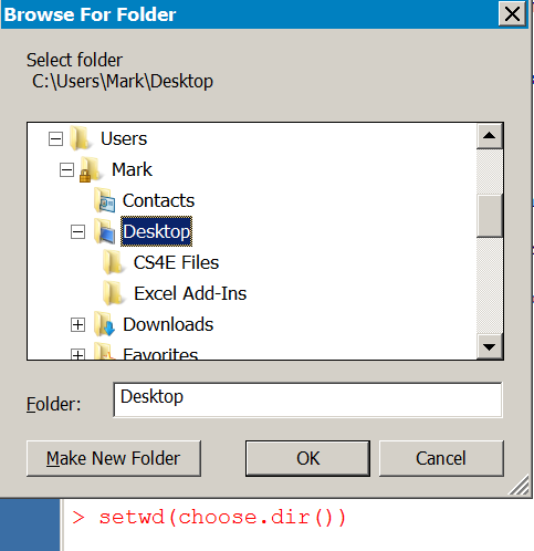
If you lot apply Windows you tin apply cull.dir() in the setwd() command to interactively set a working directory similar so:
> setwd(choose.dir())
Reading from URL
You tin can utilise scan() to read a file directly from the Internet if you accept the URL, use that instead of the filename. The URL needs to be complete and in quotes:
Annotation that you cannot use spaces in the URL. If you re-create/paste the URL from the website any spaces will be shown as %20:
> dat12 <- scan(file = "http://www.mysite/data%20files/test.txt")
Read 100 items
You tin can use all the other parameters that you've seen before. Have a become yourself using these files:
- txt – a infinite separated file
- txt – a space separated file with comments
- txt – a comma separated file
- txt – a TAB separated file
If you right-click a hyperlink you tin can re-create the URL to the clipboard.
Reading multi-column files
The browse() command reads files and stores the result as a vector. Nevertheless, many data files will contain multiple columns that correspond unlike variables. In this case you don't want a single vector particular simply a information.frame, which reflects the rows and columns of the original information.
The read.table() control is a general tool for reading files from disk (or URL) and making data.frame results. Yous can prepare decimal indicate characters and separators in a similar way to scan(). However, you lot tin can also prepare names for columns and/or rows if required.
At that place are several convenience commands to help in reading "popular" formats:
- csv() – this reads comma separated files
- csv2() – uses semi-colon as the separator and the comma as a decimal point
- delim() – uses TAB as a separator
- delim2() – uses TAB as a separator and comma as decimal signal
The read.csv() command is probably the virtually generally useful command every bit CSV format is the near widely used and can be saved by near programs.
The files L1.txt, L2.txt, L3.txt and L1c.txt are all ten columns (and 10 rows) in size. Previously y'all saw how the browse() control can read these files and create a single sample, as a vector object, from the data. By dissimilarity, the read.tabular array() command treats each column as a separate variable:
> dat12 <- read.table(file = "L1.txt") > dat12 V1 V2 V3 V4 V5 V6 V7 V8 V9 V10 1 34 35 33 26 35 35 35 32 38 29 ii 32 34 33 29 37 37 31 37 31 28 3 thirty 38 34 33 33 32 29 35 29 30 4 36 32 31 33 35 35 31 34 29 29 five 36 34 37 28 27 32 28 32 36 32 6 36 31 33 38 33 32 36 33 34 31 7 41 34 thirty 27 34 34 29 27 37 31 8 35 34 27 35 28 31 31 36 32 32 ix 30 33 36 34 29 33 28 34 37 34 10 34 33 31 30 36 26 29 35 34 35
In the preceding example the L1.txt file was used, this is space separated and so the default sep = " " need not be specified. Discover how R has "invented" names for the columns (the original file does not accept column names). If the data are comma separated yous can use the sep = "," parameter:
> dat13 <- read.table(file = "L2.txt", sep = ",")
Any comment lines are dealt with by the annotate.char parameter:
> dat14 <- read.table(file = "L1c.txt", sep = "", comment.char = "#")
The read.table() control assumes that in that location are no column names in the original information. You can assign names as part of the read.table() control using the col.names parameter. Yous need to specify exactly the correct number of names.
> cn = paste("X", ane:10, sep = "") # Make some names > cn [1] "X1" "X2" "X3" "X4" "X5" "X6" "X7" "X8" "X9" "X10" > dat15 <- read.table(file = "L1.txt", col.names = cn) > caput(dat15, n = 3) X1 X2 X3 X4 X5 X6 X7 X8 X9 X10 1 34 35 33 26 35 35 35 32 38 29 2 32 34 33 29 37 37 31 37 31 28 3 thirty 38 34 33 33 32 29 35 29 30 You lot tin always alter the names later on if you lot prefer.
Column headings
In most cases your data will contain column headings. You lot tin set these cavalcade headers using header = TRUE in the read.table() command.
> dat16 <- read.table(file = "L6.txt", header = TRUE) > dat16 Smpl1 Smpl2 Smpl3 Smpl4 Smpl5 Smpl6 Smpl7 Smpl8 Smpl9 Smpl10 i 34 35 33 26 35 35 35 32 38 29 ii 32 34 33 29 37 37 31 37 31 28 3 thirty 38 34 33 33 32 29 35 29 30 four 36 32 31 33 35 35 31 34 29 29 five 36 34 37 28 27 32 28 32 36 32 6 36 31 33 38 33 32 36 33 34 31 7 41 34 30 27 34 34 29 27 37 31 8 35 34 27 35 28 31 31 36 32 32 9 30 33 36 34 29 33 28 34 37 34 10 34 33 31 xxx 36 26 29 35 34 35
The file L6.txt is space separated. If y'all have TAB or comma separated you simply change the sep parameter as appropriate. Endeavour the following files for yourself:
- txt – a comma separated file
- txt – a TAB separated file
- txt – a space separated file
Use "\t" to represent a TAB character:
> dat17 <- read.table(file = "L5.txt", header = TRUE, sep = "\t")
Note that R will cheque to meet that the cavalcade names are "valid", and will alter the names as necessary. Y'all tin can over-ride this process using the check.names = False parameter. This can exist useful to allow numbers to be used as headings (such as years, due east.g. 2001, 2002). Nonetheless, it is a good idea to check the original datafile beginning.
Sometimes your data will have row headings, if so you will need an additional parameter, row.names.
Row headings
If your data contains row headings you can use the row.names parameter to instruct the read.tabular array() command which column contains the headings (usually the first).
> dat18 <- read.table(file = "L7.txt", sep = "", header = True, row.names = 1) > dat18 Smpl1 Smpl2 Smpl3 Smpl4 Smpl5 Smpl6 Smpl7 Smpl8 Smpl9 Smpl10 Obs1 34 35 33 26 35 35 35 32 38 29 Obs2 32 34 33 29 37 37 31 37 31 28 Obs3 xxx 38 34 33 33 32 29 35 29 thirty Obs4 36 32 31 33 35 35 31 34 29 29 Obs5 36 34 37 28 27 32 28 32 36 32 Obs6 36 31 33 38 33 32 36 33 34 31 Obs7 41 34 xxx 27 34 34 29 27 37 31 Obs8 35 34 27 35 28 31 31 36 32 32 Obs9 30 33 36 34 29 33 28 34 37 34 Obs10 34 33 31 thirty 36 26 29 35 34 35
Notice that the default is sep = "", this is used for space separated files merely yous do not need to put a infinite between the quotes! The row.names parameter needs a single numerical value, to identify the column that contains the headings. If the separator graphic symbol is unlike you simply change the sep parameter. Try the following files for yourself:
- txt – a space separated file
- txt – a comma separated file
- txt – a TAB separated file
All these files comprise both row and cavalcade names.
Usually you give a column number in the row.names parameter. Nevertheless, there are several ways to specify the row headings:
- A number corresponding to the column containing the names
- The proper noun of the column header (in quotes) containing the names
- A vector of names to use equally row headings/names
If the data are uncomplicated infinite delimited and contain column headings in all columns except the first (and then column 1 is 1 element shorter than the other columns) it volition be treated as a column of row headings (that is y'all practice not need to specify row.names). In exercise it is all-time to utilise a definite value for row.names. You can "force" simple numbered rows by setting row.names = NULL.
The read.xxx() convenience commands
There are four convenience functions, designed to make things a scrap easier when dealing with some common formats.
- csv() – this reads comma separated files
- csv2() – uses semi-colon as the separator and the comma every bit a decimal point
- delim() – uses TAB equally a separator
- delim2() – uses TAB as a separator and comma as decimal point
All these commands have header = TRUE and comment = "", prepare as default. This makes things simpler, the following commands achieve the aforementioned outcome:
> read.csv("L8.txt", row.names = ane) > read.table("L8.txt", sep = ",", header = TRUE, row.names = ane) > read.delim2("L8.txt", sep = ",", header = TRUE, row.names = ane, dec = ".") Y'all utilise whatever of the read.xxxx() commands as long every bit you over-ride the defaults. See the help entry for read.tabular array() past typing assistance(read.tabular array) in R.
Cavalcade formats
When you read a multi-column file into R the various columns are "inspected" and converted to an appropriate blazon. Generally, any character columns are converted to factor variables whilst numbers are kept as numbers. This is usually an acceptable process, since in about analytical situations y'all desire graphic symbol values to be treated as variable factors.
However, at that place may be times when you want to alter the default behaviour and read columns in a particular format. Here is a data file with several columns:
count treat day int obs1 23 how-do-you-do mon 1 obs2 17 hello tue 1 obs3 sixteen hi wed i obs4 14 lo mon two obs5 11 lo tue 2 obs6 nineteen lo wed 2
The first column tin can act as row headers/names. The "count" column is fairly evidently a numeric value. The "treat" column is an experimental factor whilst "day" is simply a characterization (text). The "int" column is intended to exist a handling label. Information technology is common in some branches of science to use plain numerical values as treatment labels.
When yous read this file into R the columns are "interpreted" like so:
> df1 <- read.csv("L11.txt", row.names = 1) > df1 count care for day int obs1 23 hi mon 1 obs2 17 hullo tue 1 obs3 sixteen hello wed one obs4 xiv lo mon 2 obs5 11 lo tue two obs6 xix lo wed 2 > str(df1) # Examine object structure 'data.frame': 6 obs. of 4 variables: $ count: int 23 17 sixteen 14 11 nineteen $ treat: Gene w/ two levels "hi","lo": 1 1 1 2 2 2 $ mean solar day : Cistron w/ three levels "mon","tue","midweek": 1 two 3 1 2 3 $ int : int ane 1 1 ii 2 2
The file L11.txt now appears to accept the cavalcade "day" converted to a factor variable and the "int" column is a number rather than a gene.
You can command the interpretation in several ways using parameters in the read.xxxx() commands:
- stringsAsFactors – set this to FALSE to proceed character columns as grapheme variables
- is – give the column numbers to keep "as is" and not convert
- colClasses – requite a vector of character strings corresponding to the classes required
The stringsAsFactors parameter is the most "simple" and is over-ridden if ane of the others is used. Information technology provides "coating coverage" and operates on the unabridged data file beingness read:
> df2 <- read.csv("L11.txt", row.names = 1, stringsAsFactors = Simulated) > str(df2) 'information.frame': six obs. of iv variables: $ count: int 23 17 xvi 14 11 19 $ care for: chr "hi" "howdy" "hi" "lo" ... $ solar day : chr "mon" "tue" "wed" "mon" ... $ int : int 1 1 1 two two 2
The equally.is parameter operates only on the columns you specify – don't forget that the cavalcade containing row names is cavalcade 1:
> df3 <- read.csv("L11.txt", row.names = 1, as.is = 4) > str(df3) 'data.frame': 6 obs. of four variables: $ count: int 23 17 16 14 11 19 $ treat: Factor westward/ two levels "hi","lo": 1 one one 2 2 two $ twenty-four hours : chr "mon" "tue" "wed" "mon" ... $ int : int ane 1 1 ii 2 2 All other parameters piece of work as they did before so if yous have a space or TAB separated file for example you lot tin use the sep parameter as necessary. Try these files if you desire some practice:
- txt – a TAB separated file with row names
- txt – a comma separated file with row names
- txt – a space separated file with row names
Using the colClasses parameter gives you the finest control over the columns. Y'all must specify (as a character vector) the required class for each cavalcade. In the example here y'all would want "count" to be an integer (or simply numeric), "treat" to be a gene, "24-hour interval" to be character and "int" to be a factor (remember we said this represented an experimental treatment). Don't forget the column of row names – apply character for these:
## Define the cavalcade classes > cc <- c("character", "integer", "factor", "character", "factor") ## Read the file and set column classes > df4 <- read.csv("L11.txt", row.names = 1, colClasses = cc) > str(df4) 'data.frame': six obs. of four variables: $ count: int 23 17 xvi xiv eleven 19 $ treat: Cistron w/ two levels "hi","lo": 1 one 1 ii two 2 $ 24-hour interval : chr "mon" "tue" "wed" "mon" ... $ int : Gene w/ 2 levels "one","ii": ane ane 1 2 ii ii You can of course ready the columns of the resulting data.frame later but information technology makes sense to exercise this right at the start.
Reading R objects from disk
R objects tin be stored on disk in 1 of ii formats:
- Binary – usually .RData files that are encoded and just readable by R
- Text – plain text files that can be read past text editors (and R)
Generally speaking an R object is something you see when you apply the ls() command, the objects() command does the same thing and the two are synonymous. Any R object tin be saved to disk.
Usually text files will be "raw information" files and scripts (collections of R commands that are executed when the script is run). However, it is possible to have text versions of other R objects.
Binary files are generally used to proceed custom commands, data and results objects. Often you'll have several objects bundled together.
There are several ways to get these objects into R.
Employ the OS to open R objects
In Windows and Mac you tin can commonly open .RData and .R files directly from the operating system. Ordinarily .RData files are associated with R so if you double click a file it will open up R and load the objects it contains. There are 2 scenarios:
- R is already running
- R is not running
You get a different result in each case.
If R is not running
If R is not running and yous double click a .RData file, R will open up and read the objects contained in the file. In improver, the working directory will be fix to the folder containing the .RData file.
And so, if yous double click the file or drag its icon to the R plan icon (shortcut on desktop, taskbar or dock) and so R volition open. You can check the working directory, which should betoken to the folder containing the file y'all opened:
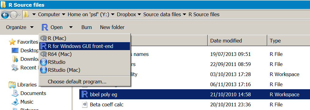
> getwd() [1] "Y:/Dropbox/Source data files/R Source files"
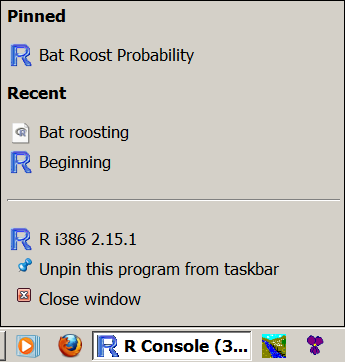
In Windows if you elevate the icon to the R program icon you tin can "pin" it to the taksbar, this can allow you lot to open a information file later with a right click of the taskbar icon:
Files that are stored in text format, commonly with the .R extension, are handled differently. Since they are plain text the default programme may well be a text editor, depending what is installed on your figurer. Y'all can correct click a file or (in Windows) click theOpen push on the card bar to see what programs are available.
In Windows you will probably take to open up the file with a text editor of some kind. If yous have the RStudio IDE yous tin can select to open the file in this, RStudio volition run and your file will appear in the script window. Note that if R has saved a text representation of objects the file volition accept Unix-mode EOL characters (LF), and Notepad will not brandish the data properly. Wordpad or Notepad++ are fine though.
In Mac you may have the file associated with a text editor or with R. If you open up the file using R then the text appears in the script editor window.
If y'all utilise Linux y'all cannot open up .RData files from the OS. R text files tin be opened in a text editor. If you apply RStudio IDE then .RData or .R files can be opened (in RStudio) from the OS.
So, .RData objects can be read into R direct via the Os but text representations of R objects (.R files) cannot.
If R is already running
If R is already running when you try to open an .RData file by double clicking, what happens depends on the Os.
- In Windows R opens in a new window
- In Mac R appends the data to the current workspace
In Windows you get another R window, the data in the .RData file is loaded and the working directory set to the binder containing the file, simply as if R had not been open.
In Mac the data are appended to the current workspace and the working directory remains unchanged.
If you are using Windows and want to suspend the information to your electric current workspace so you must drag the file icon to the running R program window and driblet information technology in. If you drag to the taskbar and expect a second, the programme window will open and you tin drop the file into the console.
Something similar happens on a Mac, yous can drag a file to the dock icon or into the running R console window.
Get binary files with load() command
Y'all tin load .RData files directly from within R using the load() command. You need to supply the proper noun of the file (in quotes) although in Windows or Mac you lot can use file.choose() instead. Any filenames must include the total file path if the file is non in your working directory.
> ls() character(0) > load(file = "Obj1.RData") > ls() [one] "data_item_1" "data_item_2"
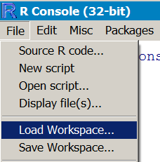
In Windows and Mac y'all tin can also use a menu:
- Mac:Workspace > Load Workspace File…
- Win:File > Load Workspace…
The data are appended to anything in the current workspace and any items that are named the aforementioned as incoming items are overwritten without warning. The working directory is unaffected.
If yous want a practice file, effort the Obj1.RData file. You lot'll have to download it, although you could endeavour loading the file using the URL.
Get text files with dget() or source() command
R can make text representations of objects. By and large, in that location are ii forms:
- Un-named objects
- Named objects
Yous'll demand to utilise the dget() or source() commands to read these text files into R.
Un-named R objects as text
Un-named objects are created using the dput() command and are text representations of unmarried objects. The text can expect slightly odd, see the D2.R instance:
structure(c(1L, 1L, 1L, 2L, 2L, 2L), .Characterization = c("high", "depression" ), class = "cistron") To read i of these objects into R you lot need the dget() command. Since the object is un-named in the text file you'll need to assign a name in the workspace:
> ls() # Cheque what is in workspace character(0) > fac1 = dget(file = "D2.R") # Go object > fac1 [1] high high high depression low low Levels: high low
Annotation that there is no GUI carte du jour command that will read this kind of text object, y'all take to use dget(). Other text representations look more than like regular R commands (i.e. the objects are named), you need a different approach for these.
Named R objects as text
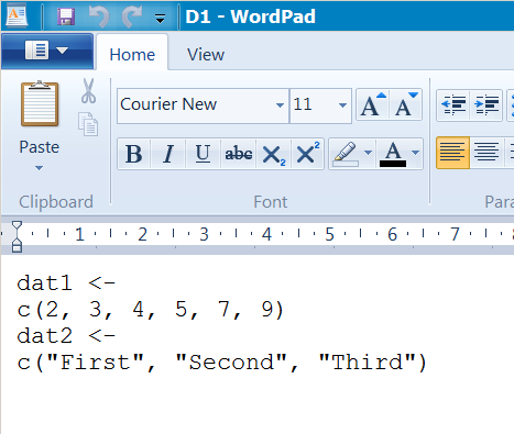
Some R text objects look more than like regular R commands. These can be saved to disk using the dump() command, which tin salve more than ane object at a time (unlike the dput() command). An example is the D1.R file:
dat1 <- c(two, three, 4, 5, 7, 9) dat2 <- c("Commencement", "Second", "Third") The D1.R file was created using the dump() command to salvage ii objects (dat1 and dat2).
To become these into R you need the source() command:
> ls() # Check what is in workspace character(0) > source(file = "D1.R") # Get the objects > ls() [ane] "dat1" "dat2" > dat1 ; dat2 [i] 2 3 4 5 seven 9 [1] "First" "2d" "3rd"
In the preceding example the file was named explicitly merely in Windows or Mac you can use file.choose() instead (also in Linux if yous are running the RStudio IDE). Find that y'all do not need to name the objects, the information file already has assigned names.
It is possible to apply menu commands in Windows or Mac to get this kind of file into R:
- Win:File > Source R code…
- Mac:File > Source File…
This kind of text file is more like a series of R commands, which would generally be called an R script. Such script files are very useful, as you can use them for many purposes, such as making a custom adding that can be run whenever you lot desire.
R script files
R script files are simply a series of R commands saved in a plain text file. When you apply the source() command, the commands are executed as if you lot had typed them into the R panel directly.
Generally speaking you'll want to "look over" the script before yous it. This usually means opening the file in a text editor. Some text editors "know" the R syntax and can highlight the text accordingly, making the script easier to follow. Both Windows and Mac R GUI have a script editor but only the Mac version has syntax highlighting.
To open a script file in the R GUI use theFile menu:
- Win:File > Open script…
- Mac:File > Open up Document…
You tin open a script in any text editor of class. In Windows the Notepad++ program is a elementary editor with syntax highlighting. On the Mac the BBEdit program is highly recommended. On Linux in that location are many options, the default text editor will frequently support syntax highlighting, Geany is i IDE that not just has syntax highlighting simply integrates with the terminal.
The RStudio IDE is very capable and makes a good platform for using R for whatsoever OS. The script editor has syntax highlighting.
If y'all start to get serious about R coding, and so the Sublime Text editor is worth a look. This has versions for all Os and syntax highlighting for R and many other languages.
Reading other types of file
R cannot read other file types "out of the box" merely at that place are command packages that will read other files. 2 commonly used ones arestrange andxlsx.
Package foreign
Theforeign package can read files created by several programs including (but not express to):
- SPSS – files fabricated past salvage or consign can be read
- dBase – .dbf files, which are also used by other programs in the XBase family
- MiniTab – .mtp MiniTab portable worksheets
- Stata – .dta files up to version 12
- Systat – .sys or .syd files
- SAS – XPORT format files (there is also a command to convert SAS files to XPORT format)
At that place are various limitations, the package has not been updated for a while. In general, it is all-time to save data in CSV format, which almost programs can practise. If y'all get sent a file in an odd format, then you lot tin ask the sender to catechumen it or try the bundle and see what you lot tin can practise. The index file of the packet help should requite you a fair indication of what is available.
Package xlsx
Thexlsx packet reads Excel files. The master control is read.xlsx(), which has various options for Excel formatted files. There is as well a read.xlsx2() command, this is more than or less the same merely uses Java more heavily and is probably better for big spreadsheets.
The essentials of the command are:
read.xlsx(file, sheetIndex, sheetName = Cypher)
Yous provide the filename (file) and either a number respective to a worksheet (sheetIndex) or the name of the worksheet (sheetName = "worksheet_name"). You can use file.choose() to select the file interactively (except on Linux).
There is likewise a parameter colClasses, which you lot can utilise to force diverse columns into the class yous require. You give a character vector containing the classes yous want – they are recycled every bit necessary. In full general, you should endeavor a regular read and run across what classes upshot. If there are some "oddities" you lot can either alter them in the imported object or re-import and prepare the classes explicitly.
Source: https://www.dataanalytics.org.uk/the-3-rs-reading/
Post a Comment for "Read in Data From a Url in R"